By John Doe September 14, 2024
Summary: In this article, we will show three different examples of using SQL to calculate rolling averages in PostgreSQL.
Table of Contents
A rolling average is a metric that allows us to find trends that would otherwise be hard to detect. It is usually based on time series data. In SQL, we calculate rolling averages using window functions.
First, let’s talk about what rolling averages are and why they’re useful.
What’s a Rolling Average?
A rolling average is a calculation that lets us analyze data points by creating a series of averages based on different subsets of a data set. It’s also called a moving average, a running average, a moving mean, or a rolling mean. You’ll very often see rolling averages used in time series data to analyze trends, especially when short-term fluctuations can hide a longer-term trend or cycle.
To show an example of a rolling average in SQL, we’ll use a stock values data set. Suppose we have a table called stock_values like the one shown below:
| date_time | stock_price |
|---|---|
| 01/04/2021 17:00 | 100.00 |
| 01/05/2021 17:00 | 130.00 |
| 01/06/2021 17:00 | 90.00 |
| 01/07/2021 17:00 | 105.00 |
| 01/08/2021 17:00 | 110.00 |
| 01/09/2021 17:00 | 140.00 |
| 01/10/2021 17:00 | 87.00 |
| 01/11/2021 17:00 | 107.00 |
| 01/12/2021 17:00 | 147.00 |
| 01/13/2021 17:00 | 92.00 |
| 01/14/2021 11:00 | 110.00 |
| 01/15/2021 17:00 | 150.00 |
| 01/16/2021 17:00 | 155.00 |
| 01/17/2021 17:00 | 97.00 |
| 01/18/2021 17:00 | 112.00 |
| 01/19/2021 17:00 | 112.00 |
In the next query, we’ll demonstrate how to use SQL to calculate the moving average for the column stock_price based on the three previous values and the current stock value:
SELECT
   date_time,
   stock_price,
   TRUNC(AVG(stock_price)
         OVER(ORDER BY date_time ROWS BETWEEN 3 PRECEDING AND CURRENT ROW), 2)
         AS moving_average
FROM stock_values;
This SQL query uses the window function AVG() on a set of values ordered by date_time. The clause ROWS BETWEEN 3 PRECEDING AND CURRENT ROW indicates that the average must be calculated only using the stock_price values of the current row and the three previous rows. Then, for each row in the result set, the rolling average will be calculated based on a different set of four stock_price values. We can see this in the following formula:
rolling_average = (stock_pricerow + stock_priceprevious_row + stock_pricerow-2 + stock_pricerow-3) / 4
Here’s the result of the previous SQL query. Notice that when stock values are extremely high or low, the rolling average takes much less extreme values:
| date_time | stock_value | rolling_average |
|---|---|---|
| 01/04/2021 17:00 | 100.00 | – |
| 01/05/2021 17:00 | 130.00 | – |
| 01/06/2021 17:00 | 90.00 | – |
| 01/07/2021 17:00 | 105.00 | 106.25 |
| 01/08/2021 17:00 | 110.00 | 108.75 |
| 01/09/2021 17:00 | 140.00 | 111.25 |
| 01/10/2021 17:00 | 87.00 | 110.50 |
| 01/11/2021 17:00 | 107.00 | 111.00 |
| 01/12/2021 17:00 | 147.00 | 120.25 |
| 01/13/2021 17:00 | 92.00 | 108.25 |
| 01/14/2021 11:00 | 110.00 | 114.00 |
| 01/15/2021 17:00 | 150.00 | 124.75 |
| 01/16/2021 17:00 | 155.00 | 126.75 |
| 01/17/2021 17:00 | 97.00 | 128.00 |
| 01/18/2021 17:00 | 112.00 | 128.50 |
| 01/19/2021 17:00 | 112.00 | 119.00 |
Moving averages are widely used in financial and technical trading, such as in stock price analysis, to examine short- and long-term trends. In the next graph, we can see the stock_price curve in blue and the rolling_average curve in orange.
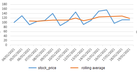
Above, we can clearly see that the rolling average has a smoother curve than the stock_price curve. Also, the running average curve shows a small uptrend that we cannot clearly see in the stock_price curve.
Using Rolling Averages to Discover Trends in New Users
Many websites use the metric “new registered users” to measure the site’s performance. In this section, we’ll use rolling averages to detect trends based on the daily count of new registered users.
Suppose we have a table called user_activity:
| user_name | action | user_type | date_time |
|---|---|---|---|
| mary1992 | user_registration | free | 2021-08-01 11:23:00 |
| john_sailor | user_registration | free | 2021-08-01 17:33:00 |
| mary1992 | passwd_change | free | 2021-08-03 01:22:00 |
| florence99 | user_registration | free | 2021-08-03 14:02:00 |
| clair2003 | user_registration | free | 2021-08-04 15:27:00 |
| sailor | upgrade_to_premium | premium | 2021-08-05 01:18:00 |
| florence99 | passwd_change | free | 2021-08-05 02:55:00 |
| andy123 | user_creation | free | 2021-08-06 12:25:00 |
As we saw in our first example, sometimes the data in the table is in the right format to calculate rolling averages. However, in the table user_activity, we need to change the format of the table data so we can work with it.
Say we want to obtain the running average of the number of new users registered each day. For this, we need a table with the columns day and registered_users. SQL has a concept called CTEs (common table expressions) that allows us to create a pseudo-table during query execution. We can then consume the CTE in the same query. Here’s an example query with a CTE:
WITH users_registered AS (
   SELECT
      date_time::date AS day,
      COUNT(*)        AS registered_users
   FROM    user_activity
   WHERE action = 'user_registration'
   GROUP BY 1
)
SELECT
  day,
  registered_users,
  TRUNC(AVG(registered_users)
        OVER(ORDER BY day ROWS BETWEEN 9 PRECEDING AND CURRENT ROW), 2)
        AS moving_average_10_days,
  TRUNC(AVG(registered_users)
        OVER(ORDER BY day ROWS BETWEEN 2 PRECEDING AND CURRENT ROW), 2)
        AS moving_average_3_days
FROM users_registered;
The previous query can be analyzed in two parts. In blue text, we have the CTE that generates a pseudo-table called users_registered; it contains the columns day and registered_users.
The second part of the query (in black text) is the calculation of the rolling average. Similarly to the first example, we use the AVG() window function and the clause OVER(ORDER BY day ROWS BETWEEN 9 PRECEDING AND CURRENT ROW). This applies the AVG() function to the current row and the nine rows before it. The query also calculates a running average for three days; the idea is to show both rolling average curves and compare how smooth they are.
The result of the previous query includes data for the last 60 days; below is a partial result set:
| day | registered_users | moving_average_10_days | moving_average_3_days |
|---|---|---|---|
| 2021-08-08 | 33 | 33.00 | 32.33 |
| 2021-08-09 | 59 | 36.30 | 39.00 |
| 2021-08-10 | 60 | 39.00 | 50.66 |
| 2021-08-11 | 75 | 43.20 | 64,66 |
| 2021-08-12 | 67 | 46.10 | 67,33 |
| 2021-08-13 | 68 | 49.70 | 70.00 |
| 2021-08-14 | 59 | 52.60 | 64,66 |
| 2021-08-15 | 65 | 55.00 | 64.00 |
| 2021-08-16 | 62 | 57.30 | 62.00 |
| 2021-08-17 | 57 | 60.50 | 61.33 |
| 2021-08-18 | 67 | 63.90 | 62.00 |
| 2021-08-19 | 63 | 64.30 | 62.33 |
| 2021-08-20 | 89 | 67.20 | 73.00 |
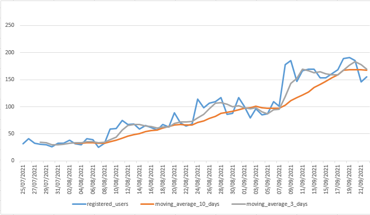
The next image shows the curves users_registered, rolling_average_10_days, and rolling_average_3_days. We can see that the curve of rolling_average_10_days (orange line) is smoother than the rolling_average_3_days curve (grey line).
The Rolling Average in Economics
In our final moving average example, we are going to analyze some economic indicators for a fictitious country. Suppose we have GDP (gross domestic product) time series data for the last 70 years. We want to know the GDP’s annual growth rate in this country and how that rate has progressed. However, in each single year there may be different factors influencing the GDP amount, such as weather, natural disasters, wars, or economic crises. Thus, we will use the rolling average GDP for 10- and 20-year periods to see the overall trend.
We have a table called yearly_gdp with the columns year and amount. Below, you can see a subset of the data from 1950 to 1965:
| year | gdp_amount |
|---|---|
| 1950 | 2396516 |
| 1951 | 1610296 |
| 1952 | 3711316 |
| 1953 | 1051886 |
| 1954 | 1113133 |
| 1955 | 2873493 |
| 1956 | 3295602 |
| 1957 | 4644432 |
| 1958 | 3312793 |
| 1959 | 2086353 |
| 1960 | 4727159 |
| 1961 | 3551490 |
| 1962 | 3282716 |
| 1963 | 3700999 |
| 1964 | 2260701 |
| 1965 | 1796435 |
The following SQL query gets the moving average of the GDP based on the last 10 and 20 years. Once again, we’ll use the AVG() window function with the OVER clause to calculate the average for the previous 10 or 20 years. Note that we use ORDER BY to ensure that the records are arranged chronologically by year:
SELECT
   year,
   gdp_amount,
   TRUNC(AVG(gdp_amount) OVER(ORDER BY year ROWS BETWEEN 9 PRECEDING AND CURRENT ROW )) AS rolling_average_gdp_10_years,
   TRUNC(AVG(gdp_amount) OVER(ORDER BY year ROWS BETWEEN 19 PRECEDING AND CURRENT ROW )) AS rolling_average_gdp_20_years
FROM yearly_gdp;
A partial result set is shown in the next image. For1950 to 1959, we don’t have a value for the 10-year rolling average; this is reasonable, since our series began in 1950 and we don’t have enough data to do a 10-year average yet. The same occurs for the 20-year running average between 1950 and 1969.
| year | gdp_amount | rolling_average_gdp_10_days | rolling_average_gdp_20_days |
|---|---|---|---|
| 1950 | 2396516 | – | – |
| 1951 | 1610296 | – | – |
| 1952 | 3711316 | – | – |
| 1953 | 1051886 | – | – |
| 1954 | 1113133 | – | – |
| 1955 | 2873493 | – | – |
| 1956 | 3295602 | – | – |
| 1957 | 4644432 | – | – |
| 1958 | 3312793 | – | – |
| 1959 | 2086353 | 2609582 | – |
| 1960 | 4727159 | 2842646 | – |
| 1961 | 3551490 | 3036766 | – |
| 1962 | 3282716 | 2993906 | – |
| 1963 | 3700999 | 3258817 | – |
| 1964 | 2260701 | 3373574 | – |
| 1965 | 1796435 | 3265868 | – |
| 1966 | 2199231 | 3156231 | – |
| 1967 | 5007340 | 3192522 | – |
| 1968 | 5570332 | 3418276 | – |
| 1969 | 4614639 | 3671104 | 3140343 |
| 1970 | 2098413 | 3408230 | 3125438 |
| 1971 | 4899398 | 3543020 | 3289893 |
| 1973 | 5943866 | 3761279 | 3416272 |
In the next graph, you can see three curves: the gdp_amount curve, the 10-year rolling average curve (which starts in 1960), and the 20-year rolling average curve. Once again, the rolling average is a smoother curve than the original raw-value curve.
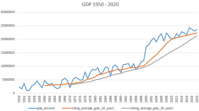
If we do the math to extract the GDP yearly growth rate from the 10-year rolling average curve, we’ll obtain values from 0–10 percent. However, if we extract the GDP yearly growth rate from the 20-year rolling average curve, we get values from 3–6 percent; the 20-year rolling average curve is smoother than the 10-year curve. Note that in 2000, the GDP had a big increase; however, the 10-year curve shows a small rise, while the 20-year curve maintains the same slope.
Finally, I would like to mention a few words about window functions. They are extremely useful when calculating metrics (as we’ve seen) and preparing reports.