September 23, 2024
Summary: Geospatial data is becoming increasingly important in many fields, from urban planning to environmental science. In this tutorial, we’ll demonstrate basic PostGIS queries for working with this type of data.
Table of Contents
Introduction to Geospatial Data and PostGIS
Geospatial data, which contains information about locations on Earth, requires specialized tools for effective use. PostGIS is a powerful PostgreSQL extension that turns a Postgres database into a full-featured Geographic Information System (GIS). With PostGIS, you can store geographic objects, run spatial queries, and perform advanced analyses directly in SQL. This makes it an essential tool for anyone working with location-based data.
Installing PostGIS allows you to perform spatial operations that usually require specialized GIS software. Whether you need to calculate distances, measure areas, or analyze spatial relationships, PostGIS equips you with the tools necessary to handle complex spatial data efficiently.
In this guide, we’ll introduce you to the basics of PostGIS. We’ll start with simple spatial queries and move on to advanced techniques like proximity analysis and network analysis.
Our Sample Geospatial Data
In this article, we’ll be working with a spatial dataset drawn from San Francisco, California. We’ll be using several tables:
-
sf_tram_stops: This table contains the locations of tram stops across the city; it also stores location coordinates and whether transfers between lines are possible at that stop. It has the following columns:id– A unique identifier for each stop.coordinates– The location coordinates of the stop.transfer_possible– If a passenger can change trams at this stop.
-
sf_planning_districts: This table defines the boundaries of San Francisco’s planning districts; this information is essential for urban analyses. It has the following columns:id– A unique identifier for each planning district.name– The district’s name.boundaries– The district’s boundaries (as location coordinates).
-
sf_bicycle_routes: This table stores information on the city’s bicycle routes; you’ll need this to analyze SanFran’s biking infrastructure. It has the following columns:id– A unique identifier for each bicycle route.course– The route’s course.condition_rating– The route’s rating (based on its conditions).
-
sf_restaurants: This table lists information on San Francisco’s restaurants, including their names, locations, ratings, and types of cuisine. It has the following columns:id– A unique identifier for each restaurant.name– The restaurant’s name.food_type– The type of cuisine served in this restaurant.rating– The restaurant’s rating.coordinates– The restaurant’s location coordinates.
-
sf_sights: This table records information on notable landmarks and points of interest (POIs) within the city. It has the following columns:id– A unique identifier for each point of interest.name– The POI’s name.coordinates– The POI’s location.
-
sf_atms: This table stores details of SanFran’s ATMs, including each ATM’s location and which company operates it. It has the following columns:id– A unique identifier for each ATM.company– The company that operates this ATM.coordinates– The ATM’s location.
This data serves as the foundation for the spatial queries we’ll be exploring. We’ll use these queries to analyze proximity between landmarks and amenities, calculate areas within planning districts, and much more. Each query will demonstrate how PostGIS helps you extract meaningful insights from spatial data.
Basic Spatial Queries with PostGIS
Once your geospatial data is stored in PostgreSQL with PostGIS, you can start querying it! Spatial queries allow you to select, filter, and manipulate data based on its location, shape, and spatial relationships. So, let’s begin working with geospatial data.
Visualizing Geospatial Data
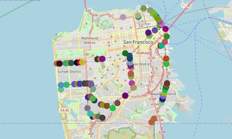
First, let’s see what geospatial data looks like. Here we select tram stop IDs and coordinates for those stops where riders can transfer:
SELECT
  id,
  coordinates
FROM sf_tram_stops
WHERE transfer_possible = true;
Here’s what the result looks like:
| id | coordinates |
|---|---|
| 1 | 0101000020E610000030D80DDB16995EC0742497FF90CE4240… |
| 4 | 0101000020E61000000DAB7823F3985EC010AFEB17ECCE4240… |
| 5 | 0101000020E6100000FDD98F1491995EC07AC7293A92CF4240… |
| … |
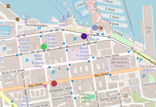
As you can see, the geospatial data in the coordinates column is not really readable. For it to be really usable, you’d need specialized software to plot it on the map. With a built-in map, you can see the location of these tram stops:
Converting Geospatial Data to Text
Maybe you want to see the location coordinates of the above tram stops without a map. You can use the following query to convert the data into human-readable coordinates:
SELECT
  id,
  ST_AsText(coordinates),
  ST_Y(coordinates),
  ST_X(coordinates)
FROM sf_tram_stops
WHERE transfer_possible = true;
This query uses the PostGIS function ST_AsText to get the coordinates in a readable format. It uses ST_Y and ST_X to extract the latitude and longitude values. Here is a partial result:
| id | st_astext | st_y | st_x |
|---|---|---|---|
| 1 | POINT(-122.39202 37.6138) | 37.6138 | -122.39202 |
| 2 | POINT(-122.38984 37.61658) | 37.61658 | -122.38984 |
| 3 | POINT(-122.39948 37.62165) | 37.62165 | -122.39948 |
| … |
Spatial Relationships
PostGIS offers several functions to explore the spatial relationships of geospatial objects. Let’s quickly review them.
ST_Intersection
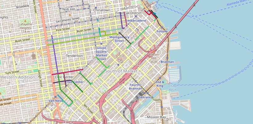
This function returns the shared part (i.e. the intersection) of two geometries. The following query shows all bicycle routes (or their parts) within the borders of the Downtown district:
SELECT
  sfbr.id,
  ST_Intersection(sfpd.boundaries, sfbr.course)
FROM sf_bicycle_routes sfbr
JOIN sf_planning_districts sfpd
  ON ST_Intersects(sfpd.boundaries, sfbr.course)
WHERE sfpd.name = 'Downtown';
The ST_Intersection function finds the area where two shapes overlap – in this case, where bicycle routes cross the boundaries of the “Downtown” district. The ST_Intersects function checks if the bicycle routes and the district boundaries touch or cross each other, making sure only those that do are included.
And here’s a partial result as text:
| id | st_intersection |
|---|---|
| 409 | 0102000020E61000000C000000438F3471DF9A5EC058F13A2… |
| 441 | 0102000020E6100000100000007451E9429B995EC0EF7A00F.. |
| 412 | 0102000020E610000009000000ED6FEAA8999A5EC06469EB2.. |
| … |
And as a map:
ST_Contains
The ST_Contains function checks if one geometry fully contains another. To list planning districts that contain ATMs from the Crown Financial company, you can run this query:
SELECT DISTINCT sfn.name
FROM sf_planning_districts sfn
JOIN sf_atms sfa
  ON ST_Contains(sfn.boundaries, sfa.coordinates)
WHERE sfa.company = 'Crown Financial Inc.';
Here’s the result:
| name |
|---|
| Downtown |
| Northeast |
ST_Within
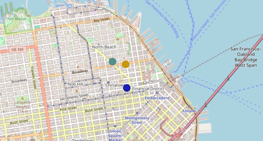
The ST_Within function also checks if one geometry is entirely within another. This query locates restaurants with a rating above 4.0 within the Northeast district:
SELECT
  sep.name,
  sep.coordinates
FROM sf_planning_districts spd
JOIN sf_restaurants sep
  ON ST_Within(sep.coordinates, spd.boundaries)
WHERE rating > 4.0
  AND spd.name = 'Northeast';
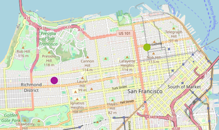
This query returns the names and coordinates of the restaurants, making them easy to visualize on a map.
| name | coordinates |
|---|---|
| Fast Duck | 0101000020E6100000B9FC87F4DB995EC02E73BA2C26E64240 |
| Red Curry | 0101000020E6100000569FABADD8995EC0E1455F419AE54240 |
| The Saloon | 0101000020E6100000D52137C30D9A5EC0431CEBE236E64240 |
Distance and Area Calculations
Calculating distances and areas is another fundamental aspect of working with geospatial data. These calculations can help answer questions like “How far is this ATM from a particular sight?” or “What is the area of this planning district?”
Distance Calculations
The ST_Distance function returns the distance between two geospatial objects. It takes two geometry arguments: ST_Distance(geometryA, geometryB).
To visualize all ATMs located within 300 meters of Fisherman’s Wharf, you can use the following query:
SELECT
  sa.id,
  sa.coordinates,
  ST_Distance(
    ST_Transform(sa.coordinates, 26910),
    ST_Transform(ss.coordinates, 26910)) AS distance
FROM sf_sights ss
JOIN sf_atms sa
  ON ST_Distance(
     ST_Transform(sa.coordinates, 26910),
     ST_Transform(ss.coordinates, 26910)) < 300
WHERE ss.name = 'Fisherman''s Wharf';
In this query, the ST_Transform function converts the given coordinates into a specific coordinate system suited for spatial calculations. The coordinate system ensures that all spatial operations (like distance calculations) are both accurate and relevant to the specific needs of the geographical area and the project.
In this query we use the coordinate system defined by the SRID (Spatial Reference System Identifier) 26910, which corresponds to the NAD83 / UTM zone 10N system. This system is commonly used for accurate distance calculations in the San Francisco area.
How can you find the right SRID? Try one of these websites:
- Spatial Reference Website: Use the EPSG tab.
- io: Type the country name, code, or coordinate system name to search and get all the possible coordinate reference systems.
- EPSG-registry.org
By transforming the coordinates, the query ensures that the distance calculation between the ATM and Fisherman’s Wharf is precise. Here’s the result:
| id | coordinates | distance |
|---|---|---|
| 132 | 0101000020E6100000FC00A436719A5EC009FEB7921DE74240 | 189.1839552624224 |
| 133 | 0101000020E61000000D897B2C7D9A5EC033A7CB6262E74240 | 277.9680083048927 |
| 135 | 0101000020E61000000E15E3FC4D9A5EC0650113B875E74240 | 216.11656973079064 |
| 136 | 0101000020E6100000910A630B419A5EC033FE7DC685E74240 | 283.89507791796825 |
Area Calculations
To calculate the area of a planning district, use the ST_Area function. This takes a geometry argument (ST_Area(geometry)) and returns the area of the resulting shape.
Here’s the query. Note that we’re using SRID = 26910 again as our coordinate system:
SELECT
  ST_Area(ST_Transform(boundaries, 26910))
FROM sf_planning_districts
WHERE name = 'Buena Vista';
And this is the result:
| st_area |
|---|
| 2617829.8666631826 |
With SRID = 26910, the default unit is meters. Thus, the result of the ST_Area is presented in square meters.
Advanced Spatial Analysis
As you become more familiar with PostGIS, you can use its advanced capabilities to perform in-depth spatial analyses. These techniques allow you to explore spatial relationships, perform proximity analyses, and even conduct network analysis – making your geospatial data insights much more actionable.
Buffering and Proximity Analysis
Buffering creates zones around spatial features. This is particularly useful in proximity analysis, where you need to determine how close certain features are to one another. For example, if you want to identify all restaurants within a 3000-meter radius of the ‘Palace of Fine Arts’, you can use the ST_DWithin function:
SELECT
  sep.name,
  sep.rating,
  sep.food_type,
  sep.coordinates,
  ST_Distance(
    ST_Transform(sep.coordinates, 26910),
    ST_Transform(ss.coordinates, 26910)) AS distance
FROM sf_sights ss
JOIN sf_restaurants sep
  ON ST_DWithin(
     ST_Transform(sep.coordinates, 26910),
     ST_Transform(ss.coordinates, 26910),
     3000)
WHERE ss.name = 'Palace of Fine Arts';
And here are your results in table and map form:
| name | rating | food_type | coordinates | distance |
|---|---|---|---|---|
| Olive | 2.10 | Greek | 0101000020E6100000C9AB730CC89A5EC0527E52EDD3E54240 | 2764.17980825426 |
| La fragranza | 4.86 | Italian | 0101000020E61000008811C2A38D9D5EC038F3AB3940E44240 | 2361.1920187470487 |
Overlay Operations
In mapping, overlay operations allow us to see how different sets of geographical information match up or interact. Imagine you have two maps, one showing all the parks in a city and another showing areas prone to flooding. By placing one map on top of the other, you can find out which parks are at risk of flooding. This process helps us to understand and visualize where different geographical features coincide; it makes planning, analyses, and decision-making more effective.
The following query uses the ST_Union function to merge the boundaries of all ‘recreational’ planning districts into a unified geometric shape:
SELECT
  ST_Union(boundaries)
FROM sf_planning_districts
WHERE type = 'recreational';
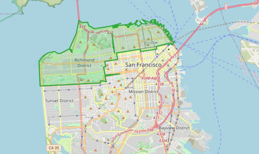
Similarly, you could use ST_Intersection to accomplish the same thing.
Network Analysis
Network analysis involves examining routes, identifying the shortest paths, and improving travel efficiency within a network. It’s critical for understanding and optimizing transportation systems and connectivity. PostGIS – when paired with pgRouting – offers robust tools for this type of analysis.
The pgRouting extension provides advanced algorithms for route optimization. One of the best-known is the pgr_dijkstra function; it computes the shortest or fastest path between two points by considering factors such as road types, traffic conditions, and other variables. This capability is invaluable for navigation systems, logistics planning, transportation management and more. By leveraging such extensions, users can enhance route planning, reduce travel times, and improve overall network efficiency.