February 29, 2024
Summary: in this tutorial, you will learn how to tune selectivity estimation of range matching.
Table of Contents
Introduction
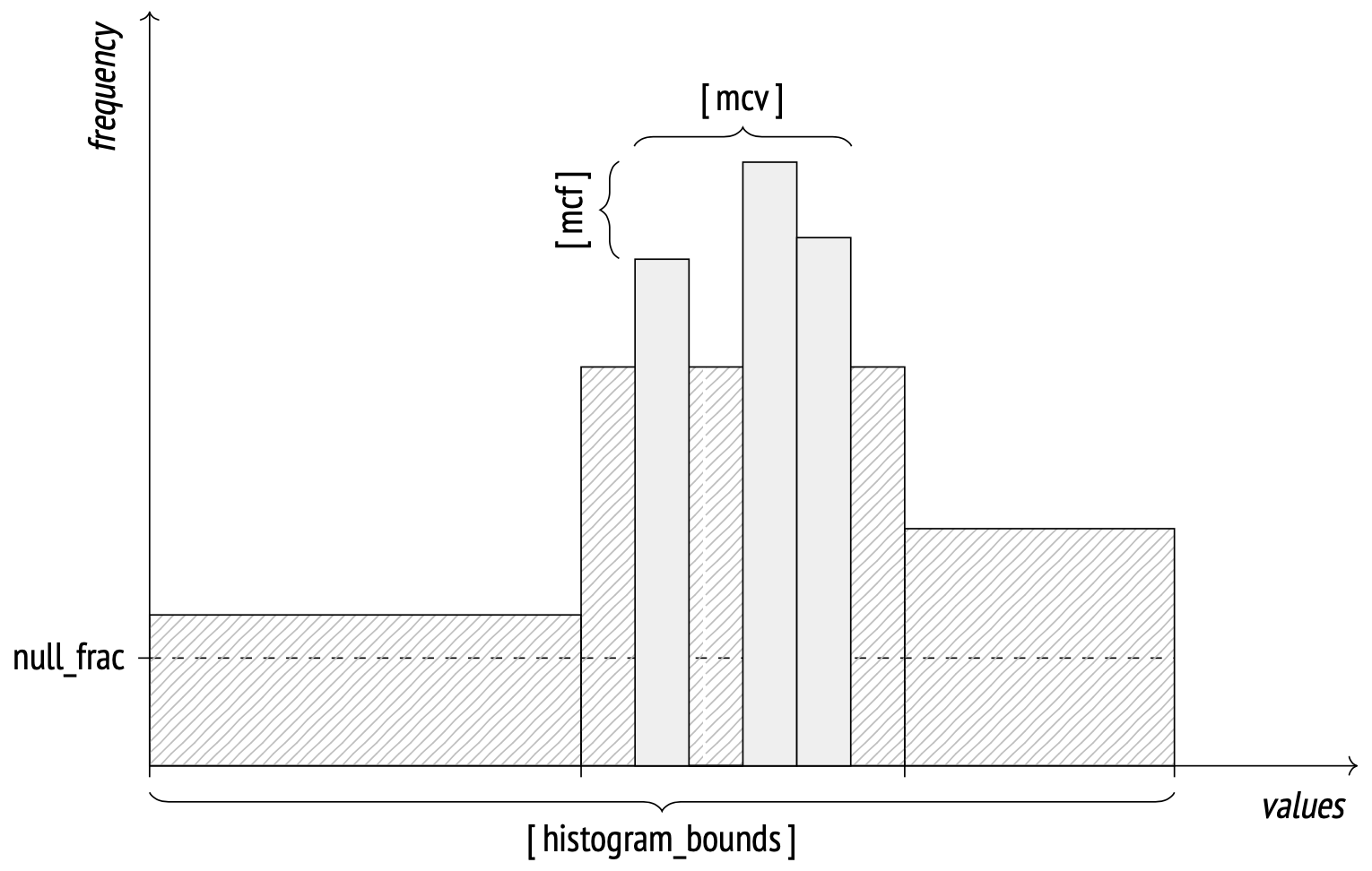
When the number of distinct values grows too large to store them all in an array, the system starts using the histogram representation. A histogram employs several buckets to store values in. The number of buckets is limited by the same default_statistics_target parameter.
The width of each bucket is selected in such a way as to distribute the values evenly across them (as indicated by the rectangles on the image having approximately the same area). This representation enables the system to store only histogram bounds, not wasting space for storing the frequency of each bucket. Histograms do not include values from MCV lists.
The bounds are stored in the histogram_bounds field in pg_stats. The summary frequency of values in any bucket equals 1 / number of buckets.
How the histogram works…
Let’s start with a little test setup:
CREATE TABLE test2 (id integer, val integer);

INSERT INTO test2 (id, val)
  SELECT i, CAST(random() * 400 AS integer)
  FROM generate_series(1, 10000) AS s(i);

ANALYZE test2;

SHOW default_statistics_target;
 default_statistics_target
---------------------------
 100
(1 row)
A histogram is stored as an array of bucket bounds:
SELECT '...' || right(histogram_bounds::text, 60) AS histogram_bounds
FROM pg_stats s
WHERE s.tablename = 'test2' AND s.attname = 'val';
                        histogram_bounds
-----------------------------------------------------------------
 ...346,350,353,357,360,364,370,374,378,382,386,389,393,397,400}
(1 row)
Among other things, histograms are used to estimate selectivity of “greater than” and “less than” operations together with MCV lists.
For example, we want to query some records from the table, filter by the column val.
EXPLAIN SELECT * FROM test2 WHERE val > 302;
                        QUERY PLAN
----------------------------------------------------------
 Seq Scan on test2  (cost=0.00..150.00 rows=2462 width=8)
   Filter: (val > 302)
(2 rows)
The cutoff value is selected specifically to be on the edge between two buckets.
The selectivity of this condition is N / number of buckets, where N is the number of buckets with matching values (to the right of the cutoff point). Remember that histograms don’t take into account most common values and undefined values.
Let’s look at the fraction of matching most common values first:
SELECT sum(s.most_common_freqs[
  array_position(s.most_common_vals::text::integer[], v)
])
FROM pg_stats s, unnest(s.most_common_vals::text::integer[]) v
WHERE s.tablename = 'test2' AND s.attname = 'val'
AND v > 302;
  sum
--------
 0.0237
(1 row)
Now let’s look at the fraction of most common values (excluded from the histogram):
SELECT sum(freq)
FROM pg_stats s, unnest(s.most_common_freqs) freq
WHERE s.tablename = 'test2' AND s.attname = 'val';
  sum
--------
 0.1442
(1 row)
There are no NULL values in the val column:
SELECT s.null_frac
FROM pg_stats s
WHERE s.tablename = 'test2' AND s.attname = 'val';
 null_frac
-----------
         0
(1 row)
The interval covers exactly 26 buckets (out of 100 total). The resulting estimate:
SELECT round( reltuples * (
   0.0237                          -- from most common values
 + (1 - 0.1442 - 0) * (26 / 100.0) -- from histogram
))
FROM pg_class WHERE relname = 'test2';
 round
-------
  2462
(1 row)
The true value is 2445.
When the cutoff value isn’t at the edge of a bucket, the matching fraction of that bucket is calculated using linear interpolation.

When the histogram data becomes outdated
Let’s check the histogram array of the column id:
SELECT '...' || right(histogram_bounds::text, 60) AS histogram_bounds
FROM pg_stats s
WHERE s.tablename = 'test2' AND s.attname = 'id';
                        histogram_bounds
-----------------------------------------------------------------
 ...900,9000,9100,9200,9300,9400,9500,9600,9700,9800,9900,10000}
(1 row)
Then insert a batch of records into the table, and query the new records from the table immediately, filter by the column id.
INSERT INTO test2 (id, val)
  SELECT i, CAST(random() * 400 AS integer)
  FROM generate_series(10001, 11000) AS s(i);

EXPLAIN (analyze) SELECT * FROM test2 WHERE id > 10000;
                                             QUERY PLAN
----------------------------------------------------------------------------------------------------
 Seq Scan on test2  (cost=0.00..168.00 rows=1 width=8) (actual time=1.527..1.752 rows=1000 loops=1)
   Filter: (id > 10000)
   Rows Removed by Filter: 10000
 Planning time: 0.115 ms
 Execution time: 1.809 ms
(5 rows)
The actual rows is 1000, while the estimated rows is 1 !
Update statistics for tables
Whenever you have significantly altered the distribution of data within a table, running ANALYZE is strongly recommended. This includes bulk loading large amounts of data into the table. Running ANALYZE (or VACUUM ANALYZE) ensures that the planner has up-to-date statistics about the table. With no statistics or obsolete statistics, the planner might make poor decisions during query planning, leading to poor performance on any tables with inaccurate or nonexistent statistics.
Note that if the autovacuum daemon is enabled, it might run ANALYZE automatically; see parameters autovacuum_analyze_threshold and autovacuum_analyze_scale_factor for more information.