June 5, 2024
Summary: in this tutorial, you will understand cost estimation for plain index scan.
Table of Contents
PostgreSQL Index Scan
Indexes return row version IDs (tuple IDs, or TIDs for short), which can be handled in one of two ways. The first one is Index scan. Most (but not all) index methods have the INDEX SCAN property and support this approach.
Let’s start with a little test setup:
CREATE TABLE events (event_id char(7) PRIMARY KEY, occurred_at timestamptz);

INSERT INTO events (event_id, occurred_at)
  SELECT to_hex(i),
  TIMESTAMP '2024-01-01 00:00:00+08' + floor(random() * 100000)::int * '1 minutes'::interval
  FROM generate_series(x'1000000'::int, x'2000000'::int, 16) AS s(i);

ANALYZE events;
The operation is represented in the plan with an Index Scan node:
EXPLAIN SELECT * FROM events
WHERE event_id = '19AC6C0' AND occurred_at = '2024-01-06 12:00:00+08';
                                  QUERY PLAN
------------------------------------------------------------------------------
 Index Scan using events_pkey on events  (cost=0.42..8.45 rows=1 width=16)
   Index Cond: (event_id = '19AC6C0'::bpchar)
   Filter: (occurred_at = '2024-01-06 04:00:00+00'::timestamp with time zone)
(3 rows)
Here, the access method returns TIDs one at a time. The indexing mechanism receives an ID, reads the relevant table page, fetches the tuple, checks its visibility and, if all is well, returns the required fields. The whole process repeats until the access method runs out of IDs that match the query.
The Index Cond line in the plan shows only the conditions that can be filtered using just the index. Additional conditions that can be checked only against the table are listed under the Filter line.
In other words, index and table scan operations aren’t separated into two different nodes, but both execute as a part of the Index Scan node. There is, however, a special node called Tid Scan. It reads tuples from the table using known IDs:
EXPLAIN SELECT * FROM events WHERE ctid = '(0,1)'::tid;
                      QUERY PLAN
-------------------------------------------------------
 Tid Scan on events  (cost=0.00..4.01 rows=1 width=16)
   TID Cond: (ctid = '(0,1)'::tid)
(2 rows)
Cost estimation
When calculating an Index scan cost, the system estimates the index access cost and the table pages fetch cost, and then adds them up.
The index access cost depends entirely on the access method of choice. If a B-tree is used, the bulk of the cost comes from fetching and processing of index pages. The number of pages and rows fetched can be deduced from the total amount of data and the selectivity of the query conditions. Index page access patterns are random by nature (because pages that are logical neighbors aren’t usually neighbors on disk too) and therefore the cost of accessing a single page is estimated as random_page_cost. The costs of descending from the tree root to the leaf page and additional expression calculation costs are also included here.
The CPU component of the table part of the cost includes the processing time of every row (cpu_tuple_cost) multiplied by the number of rows.
The I/O component of the cost depends on the index access selectivity and the correlation between the order of the tuples on disk to the order in which the access method returns the tuple IDs.
High correlation is good
In the ideal case, when the tuple order on disk perfectly matches the logical order of the IDs in the index, Index Scan will move from page to page sequentially, reading each page only once.
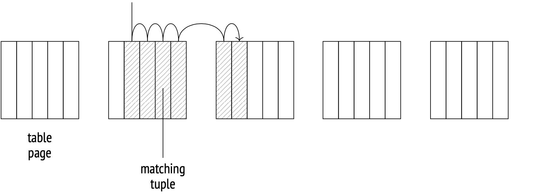
This correlation data is a collected statistic:
SELECT attname, correlation
FROM pg_stats WHERE tablename = 'events'
ORDER BY abs(correlation) DESC;
   attname   | correlation
-------------+-------------
 event_id    |           1
 occurred_at |  0.00227215
 (2 rows)
Absolute event_id values close to 1 indicate a high correlation; values closer to zero indicate a more chaotic distribution.
Here’s an example of an Index scan over a large number of rows:
EXPLAIN SELECT * FROM events WHERE event_id < '1100000';
                                    QUERY PLAN
----------------------------------------------------------------------------------
 Index Scan using events_pkey on events  (cost=0.42..2358.77 rows=73391 width=16)
   Index Cond: (event_id < '1100000'::bpchar)
(2 rows)
The total cost is about 2358.
The selectivity is estimated at:
SELECT round(73391::numeric/reltuples::numeric, 4)
FROM pg_class WHERE relname = 'events';
 round
--------
 0.0700
(1 row)
This is about 1/16, which is to be expected, considering that event_id values range from 1000000 to 2000000.
For B-trees, the index part of the cost is just the page fetch cost for all the required pages. Index records that match any filters supported by a B-tree are always ordered and stored in logically connected leaves, therefore the number of the index pages to be read is estimated as the index size multiplied by the selectivity. However, the pages aren’t stored on disk in order, so the scanning pattern is random.
The cost estimate includes the cost of processing each index record (at cpu_index_tuple_cost) and the filter costs for each row (at cpu_operator_cost per operator, of which we have just one in this case).
The table I/O cost is the sequential read cost for all the required pages. At perfect correlation, the tuples on disk are ordered, so the number of pages fetched will equal the table size multiplied by selectivity.
The cost of processing each scanned tuple (cpu_tuple_cost) is then added on top.
WITH costs(idx_cost, tbl_cost) AS (
  SELECT
    ( SELECT round(
        current_setting('random_page_cost')::real * pages +
        current_setting('cpu_index_tuple_cost')::real * tuples +
        current_setting('cpu_operator_cost')::real * tuples
      )
      FROM (
        SELECT relpages * 0.0700 AS pages, reltuples * 0.0700 AS tuples
        FROM pg_class WHERE relname = 'events_pkey'
      ) c
    ),
    ( SELECT round(
        current_setting('seq_page_cost')::real * pages +
        current_setting('cpu_tuple_cost')::real * tuples
      )
      FROM (
        SELECT relpages * 0.0700 AS pages, reltuples * 0.0700 AS tuples
        FROM pg_class WHERE relname = 'events'
      ) c
    )
)
SELECT idx_cost, tbl_cost, idx_cost + tbl_cost AS total FROM costs;
 idx_cost | tbl_cost | total
----------+----------+-------
     1364 |      989 |  2353
(1 row)
This formula illustrates the logic behind the cost calculation, and the result is close enough to the planner’s estimate. Getting the exact result is possible if you are willing to account for several minor details, but that is beyond the scope of this article.
Low correlation is bad
The whole picture changes when the correlation is low. Let’s create an index for the occurred_at column, which has a near-zero correlation with the index, and run a query that selects a similar number of rows as in the previous example. Index access is so expensive (16812 against 2358 in the good case) that the planner only selects it if told to do so explicitly:
CREATE INDEX ON events(occurred_at);
SET enable_seqscan = off;
SET enable_bitmapscan = off;

EXPLAIN SELECT * FROM events
WHERE occurred_at < '2024-01-06 12:00:00+08';
                                          QUERY PLAN
----------------------------------------------------------------------------------------------
 Index Scan using events_occurred_at_idx on events  (cost=0.42..16812.36 rows=78629 width=16)
   Index Cond: (occurred_at < '2024-01-06 04:00:00+00'::timestamp with time zone)
(2 rows)
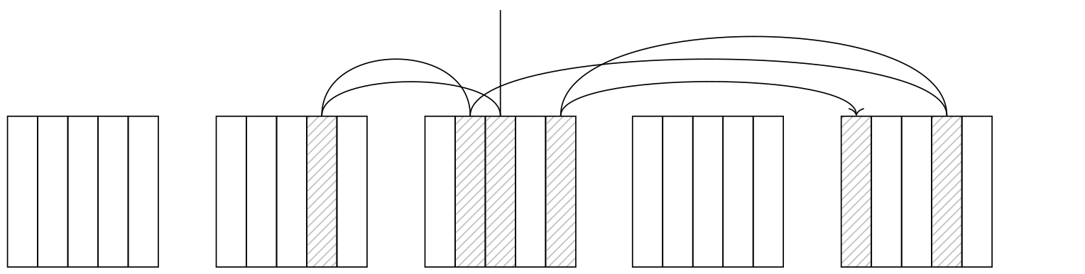
A lower correlation means that the order in which the access method returns tuple IDs will have little to do with the actual positions of the tuples on disk, so every next tuple will be in a different page. This makes the Index Scan node jump from page to page, and the number of page fetches in the worst case scenario will equal the number of tuples.
This doesn’t mean, however, that simply substituting seq_page_cost with random_page_cost and relpages with reltuples will give us the correct cost. In fact, that would give us an estimate of 316820, which is much higher than the planner’s estimate.
The key here is caching. Frequently accessed pages are stored in the buffer cache (and in the OS cache too), so the larger the cache size, the higher the chance to find the requested page in it and avoid accessing the disk. The cache size for planning specifically is defined by the effective_cache_size parameter (4GB by default). Lower parameter values increase the expected number of pages to be fetched. I won’t put the exact formula here (you can dig it up from the backend/optimizer/path/costsize.c file, under the index_pages_fetched function). What I will put here is a graph illustrating how the number of pages fetched relates to the table size (with the selectivity of 1/2 and the number of rows per page at 10):
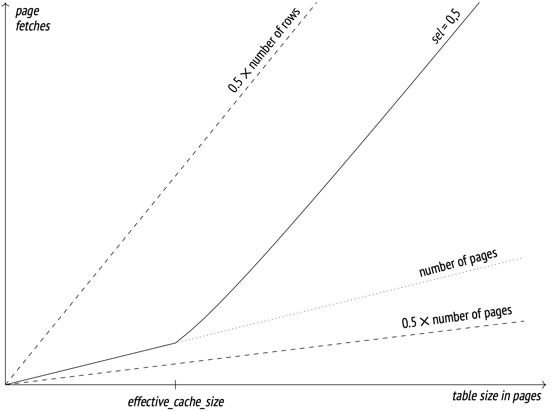
The dotted lines show where the number of fetches equals half the number of pages (the best possible result at perfect correlation) and half the number of rows (the worst possible result at zero correlation and no cache).
The effective_cache_size parameter should, in theory, match the total available cache size (including both the PostgreSQL buffer cache and the system cache), but the parameter is only used in cost estimation and does not actually reserve any cache memory, so you can change it around as you see fit, regardless of the actual cache values.
If you tune the parameter way down to the minimum, you will get a cost estimation very close to the no-cache worst case mentioned before:
SET effective_cache_size = '8kB';

EXPLAIN SELECT * FROM events
WHERE occurred_at < '2024-01-06 12:00:00+08';
                                          QUERY PLAN
-----------------------------------------------------------------------------------------------
 Index Scan using events_occurred_at_idx on events  (cost=0.42..316678.81 rows=78629 width=16)
   Index Cond: (occurred_at < '2024-01-06 04:00:00+00'::timestamp with time zone)
(2 rows)

RESET effective_cache_size;
RESET enable_seqscan;
RESET enable_bitmapscan;
When calculating the table I/O cost, the planner takes into account both the worst and the best case costs, and then picks an intermediate value based on the actual correlation.
Index Scan is efficient when you scan only some of the tuples from a table. The more the tuple locations in the table correlate with the order in which the access method returns the IDs, the more tuples can be retrieved efficiently using this access method. Conversely, the access method at a lower order correlation becomes inefficient at a very low number of tuples.