September 13, 2024
Summary: in this tutorial, you will learn some practical examples of leveraging the ROWS BETWEEN clause with window functions in PostgreSQL.
Table of Contents
Introduction
SQL window functions are tremendously useful for calculating complex aggregations like moving averages or running totals. The ROWS clause allows you to specify rows for your calculations, enabling even more sophisticated window frames. Here are five practical examples of leveraging the ROWS BETWEEN clause in SQL.
Window functions (also called OVER functions) compute their result based on a sliding window frame (i.e. a set of rows). They are similar to aggregate functions in that you can calculate the average, total, or minimum/maximum value across a group of rows. However, there are some important differences:
- Window functions do not collapse rows as aggregate functions do. Thus, you can still mix attributes from an individual row with the results of a window function.
- Window functions allow sliding window frames, meaning that the set of rows used for the calculation of a window function can be different for each individual row.
The syntax of a window function is shown below:
SELECT <column_1>, <column_2>,
  window_function(<...>) OVER (
    PARTITION BY <...>
    ORDER BY <...>
    <window_frame>) <window_column_alias>
FROM <table_name>;
When you use a window function in the SELECT statement, you basically calculate another column with this function:
-
You start by specifying a function (e.g.
AVG(),SUM(), orCOUNT()). -
Then, you use the
OVERkeyword to define a set of rows. Optionally, you can:- Group the rows with
PARTITION BYso that functions will be calculated within these groups instead of the entire set of rows. - Sort the rows within a window frame using ORDER BY if the order of rows is important (e.g. when calculating running totals).
- Specify the window frame’s relation to the current row (e.g. the frame should be the current row and two previous ones, or the current row and all the following rows, etc.).
- Group the rows with
A window frame is defined using ROWS, RANGE, and GROUPS clauses. In this article, we’ll focus on the ROWS clause and its options.
ROWS Clause: Syntax and Options
The purpose of the ROWS clause is to specify the window frame in relation to the current row. The syntax is:
ROWS BETWEEN lower_bound AND upper_bound
The bounds can be any of these five options:
UNBOUNDED PRECEDING– All rows before the current row.n PRECEDING– n rows before the current row.CURRENT ROW– Just the current row.n FOLLOWING– n rows after the current row.UNBOUNDED FOLLOWING– All rows after the current row.
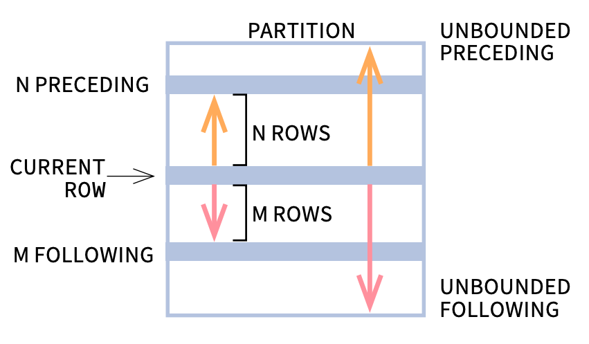
Here are a couple of things to keep in mind when defining window frames with the ROWS clause:
-
The window frame is evaluated separately within each partition.
-
The default option depends on if you use
ORDER BY:- With
ORDER BY, the default frame isRANGE BETWEEN UNBOUNDED PRECEDING AND CURRENT ROW. - Without
ORDER BY, the default frame isROWS BETWEEN UNBOUNDED PRECEDING AND UNBOUNDED FOLLOWING.
- With
-
If one of your bounds is a current row, you can skip specifying this bound and use a shorter version of the window frame definition:
UNBOUNDED PRECEDINGis the same asBETWEEN UNBOUNDED PRECEDING AND CURRENT ROW.n PRECEDINGis the same asBETWEEN n PRECEDING AND CURRENT ROW.n FOLLOWINGis the same asBETWEEN CURRENT ROW AND n FOLLOWING.UNBOUNDED FOLLOWINGis the same asBETWEEN CURRENT ROW AND UNBOUNDED FOLLOWING.
Let’s move to the examples to see how this works in practice.
Examples of Using ROWS in Window Functions
Example 1
To get started with the ROWS clause, we’ll use the following table with sales data from a book store.
Table sales
| record_id | date | revenue |
|---|---|---|
| 1 | 2021-09-01 | 1515.45 |
| 2 | 2021-09-02 | 2345.35 |
| 3 | 2021-09-03 | 903.99 |
| 4 | 2021-09-04 | 2158.55 |
| 5 | 2021-09-05 | 1819.80 |
In our first example, we want to add another column that shows the total revenue from the first date up to the current row’s date (i.e. running total). Here’s the query we can use:
SELECT date, revenue,
	SUM(revenue) OVER (
      ORDER BY date
      ROWS BETWEEN UNBOUNDED PRECEDING AND CURRENT ROW) running_total
FROM sales
ORDER BY date;
To calculate the running total using a window function, we go through the following steps:
- Calculating the total revenue using the
SUM()aggregate function. - Ordering the records in the window frame by date (the default is in ascending order), since the order of rows matters when calculating a running total.
- Specifying the window frame by defining the lower bound as
UNBOUNDED PRECEDINGand the upper bound asCURRENT ROW. This will include all rows up to and including the current one. Note that the default behavior without theROWSclause specified would be the same in this case. The default frame usesRANGE, notROWS. As each day appears only once in the table, the result will be the same forRANGEandROWS. Thus, we could also use the following query to get the same results:
SELECT date, revenue,
	SUM(revenue) OVER (
      ORDER BY date) running_sum
FROM sales
ORDER BY date;
| date | revenue | running_total |
|---|---|---|
| 2021-09-01 | 1515.45 | 1515.45 |
| 2021-09-02 | 2345.35 | 3860.80 |
| 2021-09-03 | 903.99 | 4764.79 |
| 2021-09-04 | 2158.55 | 6923.34 |
| 2021-09-05 | 1819.80 | 8743.14 |
As you see, the query worked as intended and we got the running total in our third column. On the first day, it equals the sales from this day – $1515.45; on the second day, it equals the sum of sales from the first and second days – $3860.80; in the next row, we get the sum of sales from the first three days – $4764.79, etc.
In our next examples, we’ll see how the ROWS clause works when the records are divided into several groups.
Example 2
For the next couple of examples, we’ll use the table below. It contains fictional data on average temperature (in °C) and total precipitation (in mm) in two Chinese cities (Shanghai and Beijing) over five consecutive days.
Table weather
| record_id | date | city | temperature | precipitation |
|---|---|---|---|---|
| 101 | 2021-09-01 | Shanghai | 18.5 | 7 |
| 102 | 2021-09-01 | Beijing | 17.3 | 5 |
| 103 | 2021-09-02 | Shanghai | 18.0 | 20 |
| 104 | 2021-09-02 | Beijing | 17.0 | 15 |
| 105 | 2021-09-03 | Shanghai | 20.1 | 12 |
| 106 | 2021-09-03 | Beijing | 19.0 | 10 |
| 107 | 2021-09-04 | Shanghai | 20.2 | 0 |
| 108 | 2021-09-04 | Beijing | 19.6 | 0 |
| 109 | 2021-09-05 | Shanghai | 22.5 | 0 |
| 110 | 2021-09-05 | Beijing | 20.4 | 0 |
We want to calculate the three-days moving average temperature separately for each city. To separate the calculations for the two cities, we’ll include the PARTITION BY clause. Then, when specifying the window frame, we’ll be considering the current day and the two preceding days:
Note also that we’ve put our window function inside the ROUND() function so that the three-day moving average is rounded to one decimal place. Here’s the result:
| city | date | temperature | mov_avg_3d_city |
|---|---|---|---|
| Beijing | 2021-09-01 | 17.3 | 17.3 |
| Beijing | 2021-09-02 | 17.6 | 17.5 |
| Beijing | 2021-09-03 | 19.0 | 18.0 |
| Beijing | 2021-09-04 | 19.6 | 18.7 |
| Beijing | 2021-09-05 | 20.4 | 19.7 |
| Shanghai | 2021-09-01 | 18.5 | 18.5 |
| Shanghai | 2021-09-02 | 19.0 | 18.8 |
| Shanghai | 2021-09-03 | 20.1 | 19.2 |
| Shanghai | 2021-09-04 | 20.2 | 19.8 |
| Shanghai | 2021-09-05 | 22.5 | 20.9 |
The moving average was calculated separately for Beijing and Shanghai. For September 1st, the moving average equals the average daily temperature, as we don’t have any preceding records. Then, on September 2nd, the moving average is calculated as the average temperature for the 1st and 2nd (17.5 °C in Beijing and 18.8 °C in Shanghai, respectively). On September 3rd, we finally have enough data to calculate the average temperature for three days (the two preceding and the current day), which turns out to be 18.0 °C in Beijing and 19.2°C in Shanghai. Then, the three-day moving average for Sep 4th is calculated as the average temperature for the 2nd, 3rd, and 4th, and so on.
Here’s one more thing to note: The order of records in the window frame has a key role in specifying which rows to consider.
In the query above, we have ordered the records in the window frame by date in ascending order (using the default setting), i.e. we’re starting with the earliest date. Then, to include two days before the current day in our calculations, we have set the lower bound as 2 PRECEDING.
However, we could get the exact same window frame by ordering the records in descending order, and then changing the ROWS option to include 2 FOLLOWING instead of 2 PRECEDING:
SELECT city, date, temperature,
	ROUND(AVG(temperature) OVER (
      PARTITION BY city
      ORDER BY date DESC
      ROWS BETWEEN CURRENT ROW AND 2 FOLLOWING), 1) mov_avg_3d_city
FROM weather
ORDER BY city, date;
This query outputs the exact same result.
Example 3
In this example, we’ll calculate the total precipitation for the last three days (i.e. a three-day running total) separately for two cities.
SELECT city, date, precipitation,
	SUM(precipitation) OVER (
      PARTITION BY city
      ORDER BY date
      ROWS 2 PRECEDING) running_total_3d_city
FROM weather
ORDER BY city, date;
In this query, we again partition the data by city. We use the SUM() function to calculate the total level of precipitation for the last three days, including the current day. Also, note that we use an abbreviation when defining the window frame by specifying only the lower bound: 2 PRECEDING.
Here’s the output of the above query:
| city | date | precipitation | running_total_3d_city |
|---|---|---|---|
| Beijing | 2021-09-01 | 5 | 5 |
| Beijing | 2021-09-02 | 15 | 20 |
| Beijing | 2021-09-03 | 10 | 30 |
| Beijing | 2021-09-04 | 0 | 25 |
| Beijing | 2021-09-05 | 0 | 10 |
| Shanghai | 2021-09-01 | 7 | 7 |
| Shanghai | 2021-09-02 | 20 | 27 |
| Shanghai | 2021-09-03 | 12 | 39 |
| Shanghai | 2021-09-04 | 0 | 32 |
| Shanghai | 2021-09-05 | 0 | 12 |
As of September 3rd, we get a three-day running total of precipitation in Beijing: 30 mm. This is the sum of 5 mm precipitation from September 1st, 15 mm from the 2nd, and 10 mm from the 3rd.
Do you know how we got the 12 mm running total for Shanghai on Sep 5th? Try to follow the results in our output table to make sure you understand how window functions work with specific window frames.
Now let’s move on to some new data and examples.
Example 4
For the next two examples, we’ll be using the data shown below. It includes daily information on the number of new subscribers across three social networks: Instagram, Facebook, and LinkedIn.
Table subscribers
| record_id | date | social_network | new_subscribers |
|---|---|---|---|
| 11 | 2021-09-01 | 40 | |
| 12 | 2021-09-01 | 12 | |
| 13 | 2021-09-01 | 5 | |
| 14 | 2021-09-02 | 67 | |
| 15 | 2021-09-02 | 23 | |
| 16 | 2021-09-02 | 2 | |
| 17 | 2021-09-03 | 34 | |
| 18 | 2021-09-03 | 25 | |
| 19 | 2021-09-03 | 10 | |
| 20 | 2021-09-04 | 85 | |
| 21 | 2021-09-04 | 28 | |
| 22 | 2021-09-04 | 20 |
Let’s start by calculating the running totals for the number of new subscribers separately for each network. Basically, for each day, we want to see how many people have subscribed since we started collecting data until the current row’s date.
Here’s an SQL query that meets this request:
SELECT social_network, date, new_subscribers,
	SUM(new_subscribers) OVER (
      PARTITION BY social_network
      ORDER BY date
      ROWS UNBOUNDED PRECEDING) running_total_network
FROM subscribers
ORDER BY social_network, date;
We start by calculating the total number of new subscribers using the SUM() aggregate function. Then, we use the PARTITION BY clause to compute separate calculations for each network. We also sort the records by date in the ascending order (by default). Finally, we define the window frame as UNBOUNDED PRECEDING to include all records up to the current one inclusively.
The output looks like this:
| date | social_network | new_subscribers | running_total_network |
|---|---|---|---|
| 2021-09-01 | 12 | 12 | |
| 2021-09-02 | 23 | 35 | |
| 2021-09-03 | 25 | 60 | |
| 2021-09-04 | 28 | 88 | |
| 2021-09-01 | 40 | 40 | |
| 2021-09-02 | 67 | 107 | |
| 2021-09-03 | 34 | 141 | |
| 2021-09-04 | 85 | 226 | |
| 2021-09-01 | 5 | 5 | |
| 2021-09-02 | 2 | 7 | |
| 2021-09-03 | 10 | 17 | |
| 2021-09-04 | 20 | 37 |
In the results table, you can see how the number of new subscribers is added to the cumulative total for each new record. The running total is calculated separately for each network, as specified in the window function.
Example 5
In our final example, I want to demonstrate how we can display the first and the last value of a specific set of records using window functions and the ROWS clause. This time, let’s add two columns to the output:
- The number of new subscribers added on the first day, and
- The number of new subscribers added on the last day.
With this information calculated separately for each social network, we can see how every day’s performance compares to where we’ve started and where we are now.
Here’s the SQL query to get the required output:
SELECT social_network, date, new_subscribers,
    FIRST_VALUE(new_subscribers) OVER(
      PARTITION BY social_network
      ORDER BY date) AS first_day,
    LAST_VALUE(new_subscribers) OVER(
      PARTITION BY social_network
      ORDER BY date
      ROWS BETWEEN UNBOUNDED PRECEDING AND UNBOUNDED FOLLOWING) AS last_day
FROM subscribers
ORDER BY social_network, date;
As you see, we are using the FIRST_VALUE() and the LAST_VALUE() functions to get the information on the first and the last days, respectively. Note also how we specify the window frame for each of the functions:
- We don’t include the ROWS clause with the FIRST_VALUE() function because the default behavior (i.e.
RANGE BETWEEN UNBOUNDED PRECEDING AND CURRENT ROW) is fine for our purposes. - However, we do specify the window frame with the
LAST_VALUE()function because the default option would use the current row value as the last value for each record; this is not what we are looking for in this example. We specify the window frame asROWS BETWEEN UNBOUNDED PRECEDING AND UNBOUNDED FOLLOWINGto make sure all records are considered.
And here’s the result set:
| date | social_network | new_subscribers | first_day | last_day |
|---|---|---|---|---|
| 2021-09-01 | 12 | 12 | 28 | |
| 2021-09-02 | 23 | 12 | 28 | |
| 2021-09-03 | 25 | 12 | 28 | |
| 2021-09-04 | 28 | 12 | 28 | |
| 2021-09-01 | 40 | 40 | 85 | |
| 2021-09-02 | 67 | 40 | 85 | |
| 2021-09-03 | 34 | 40 | 85 | |
| 2021-09-04 | 85 | 40 | 85 | |
| 2021-09-01 | 5 | 5 | 20 | |
| 2021-09-02 | 2 | 5 | 20 | |
| 2021-09-03 | 10 | 5 | 20 | |
| 2021-09-04 | 20 | 5 | 20 |
As requested, we have the number of new subscribers on the first and the last day calculated separately for each social network.